In this series of posts on position sizing using the Percent Risk per Trade model, this week I will explain how to use a more scientific approach to determine what Stop Loss to use to determine the Dollar Risk per Share or the Trade Risk. The objective is to overcome the problems highlighted in last week’s posting.
Some of the key requirements regarding where to place the Stop Loss are to determine:
- The timeframe of the trading approach; ultra-short, short, medium or long term.
- The current characteristics of the stock / instrument in which a position is about to be taken. This gives the trader a deep insight into how the price action might react in the future.
- The cycle that the price action is in when the set up or signal that reacts to the current price action occurs. For example, is the price action oversold or exhausted to the downside, overbought or exhausted to upside, a breakout or in a sideways pattern?
Let’s cover these three requirements.
Timeframe: The SPA3 system that I designed during the 1990’s and released for commercial use in 1998 is a medium term approach for trading equities on the ASX, JSE and NASDAQ (and CFDs on the ASX).
All active investors need to be objective about the timeframe in which any of their trading approaches trades. That is, the timeframe in which they expect the rising trend may end on the upside, and in which their open position needs to be closed on the downside because the anticipated price rise has not materialised and has done the opposite, fallen. Timeframe will determine the sensitivity of entry and exit criteria including what data to use: intraday, daily, weekly and/or monthly.
Characteristics: Stocks display changing characteristics at different times depending on stock specific news, company performance, market conditions, sector conditions, economic conditions, economic news or geopolitical news. A method is needed to determine a stock’s current characteristics. Various technical analysis techniques can be used to assess these including the stock’s current price volatility, which I believe to be the most effective.
Price Cycle: Technical analysis is the investment tool to use to determine where a stock, index or commodity is in its current cycle of price action. There is no other way! Even fundamental analysts need to know where price currently is relative to its past when calculating most of their fundamental analysis ratios.
Using technical analysis in the timeframe in which you trade, measure the characteristics and positioning of price action in the current cycle. This can be done in one of two ways, using:
- discretion, such as I did in last week’s posting in determining where to place a Stop Loss, or
- a rules-based, unambiguous and non-discretionary method. The latter is also called a mechanical method and this is what I use and have used for over one and half decades.
When using a mechanical method, objective research can be conducted to find answers to those questions posed in the postings over the last 2 weeks because an unambiguous method can be objectively defined to a computer which can be programmed with many ‘what if’ scenarios that can then be stress tested under many different market conditions to determine the answers that are sought.
It is impossible to conduct research using a discretionary approach because such a method cannot be programmed into a computer. You see, the computer needs to know PRECISELY how to react in any given situation in the past, without any discretion whatsoever, and, once discovered, that needs to be how the trader will react in the future when the same criteria are met.
I need readers to understand how important the role of a mechanical system plays in being able to conduct such research because research is the key to determining an objective Trade Risk.
With SPA3 a technical Stop Loss is not defined at the outset of the trade (but the Trade Risk is – I will get to this in a moment). SPA3 has a number of different technical exits including:
- Profit Stop exits, which are targets established at the outset of the trade based on the characteristics of the stock.
- Momentum exits based on weekly and daily data using the SIROC indicator.
- Volatility exits for highly volatile price action.
These exits are mechanical, meaning that there is no wiggle room for discretion on why or when to act, the trader simply acts when the criteria are met. Period! Once.….
- the entries and exits are defined objectively and unambiguously, and
- it is established that trading with these entries and exits the trader will have a statistical edge in the market because the unambiguous entries and exits have been:
- researched over many thousands of historical trades, and
- researched over tens of thousands of walk-forward trades, and
- live-traded in thousands of trades,
-
……then quantitative analysis can be conducted on tens of thousands of trades to correlate, amongst many other things, the expected loss per trade for different types of price action, as determined by the volatility of the price action and the cycle of the price action.
This expected loss per trade is used as the ‘Stop Loss’, or Trade Risk, in the Percent Risk per Trade position size calculation and is different for each and every trade based on the quantitative analysis research outcomes for the then current price action for any given stock. Rather than the Stop Loss being a technical Stop Loss it is a quantitative Stop Loss.
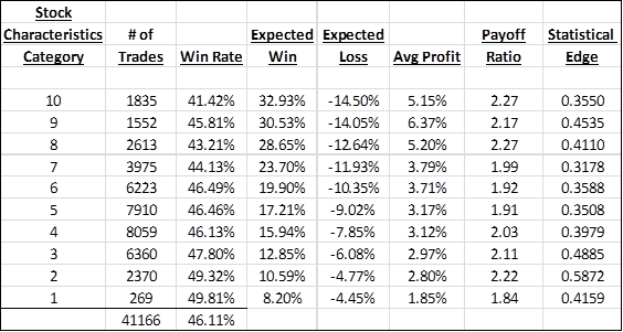
To give the reader an idea, this table shows the respective quantitative Stop Loss’s for 10 categories of different stock characteristics on the NASDAQ. However, when the Trade Risk is calculated for SPA3 it is even more specific as a smoothed curve has been created for calculating the Trade Risk for all volatility readings correct to 3 decimal points, rather than using a ‘stepped’ calculation based on grouped categories.
Position sizing software (a spreadsheet could be used) has been developed that stores the necessary quantitative information in a Risk Table to determine the Trade Risk which is then applied when the entry criteria are met for any given stock at any given time. Here is an example:
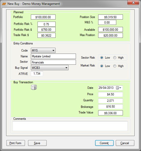
The quantitative, or expected, Stop Loss for this trade alongside the “Trade Risk $” box is $0.3622, or 36.22 cents. For the characteristics of this stock for its current price cycle action this is the quantitative Stop Loss used purely for the position size calculation.
And that’s how we calculate the Trade Risk. In essence we have turned the equation around and let research, via quantitative analysis, tell us where to place the expected Stop Loss rather than subjectively determine where to place a technical Stop Loss using eye-ball technical analysis. This is one of the beauties of using a mechanical approach. It is scientific. It is rigorous. It is structured. And multiple ‘what if’ scenarios can be modelled.
So what? How do we know that this works and is better than using another approach? Well, firstly, it has to work at a practical level, it has to be executable in the market and it has to demonstrate that it’s profitable.
So we know how to calculate our Trade Risk for the Percent Risk per Trade model. The next two big questions are:
- “What Percent Risk per Trade do I use? 2%, 3%, 1.5%, 1%, 0.5%? This question was answered in some detail in my posting a few weeks ago on March 21 “Busting the Myth of the 2% Rule“.
- “How do we know that the edge combined with its position sizing even works in a portfolio at all, and if it does, what the life journey of that portfolio would look like under different market conditions?
These are the really juicy bits. The second question will be covered in next week’s posting.