One step ahead – New groundbreaking Research Part 8

From the Share Wealth Systems R&D Team

_
System Quality Number

Before I take you through the statistical differences of the Pre December 2011 SPA3 Edge versus the Revised Edge, I need you to understand an important step forward I made while on this journey. While it’s not entirely new in the realms of measuring statistics and systems design, it played a major role in helping to achieve our predefined research objectives.

If you remember, our two core objectives at the start of this process were to:

• • Increase returns
  • Reduce drawdown

To achieve these objectives, we first needed to make each trade more similar to one another. As stated in a previous blog post, the more similar individual trade outcomes are, the more flexibility one has with their money management. This then increases the probability of limiting drawdown and increasing returns in their portfolios.

Ralph Vince made the statement, “The most important preparation a trader can do is to make as certain as possible that he has a positive mathematical expectation in the future”. While I am a big believer that every investor must trade and invest with an Edge – expectancy is a calculation that determines whether an edge is present or not – it does not measure the variability of outcomes of trades that comprise the edge.

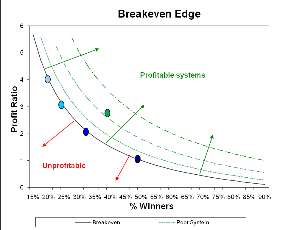
So what is SPA3’s edge? In the graph above, all the blue dots are on the breakeven line of the Expectancy curve, i.e. an Expectancy of 0. This is calculated using the formula, Expectancy = [(Profit Ratio + 1) * Win Rate] – 1. The green dot is where SPA3 without Risk Tables (prior to this round of research) is positioned on the Expectancy curve with a Profit Ratio of around 2.7 and a Win Rate of around 40% resulting in an Expectancy of around 0.48 = [(2.7 + 1) * 0.4] – 1.

Thomas Stridsman in his book “Trading Systems that Work” takes this concept expectancy even further. He points out: “The point is, by keeping the standard deviation of outcomes lower, while at the same time also decreasing the ratio between the open profits and closed out profits, we can be more aggressive (and flexible) when it comes to position sizes traded in our portfolio, according to a fixed fractional trading strategy.”

So far in this series of blogs we have discussed reducing End of Trade Drawdown which is the same as “decreasing the ratio between the open profits and closed out profits” that Stridsman refers to.

In order to test and determine whether we can keep the “standard deviation of outcomes lower”, firstly all trade outcomes must be expressed in terms of the risk taken on each trade. This could be the distance to an initial stop for each trade or could be the average loss per trade as measured over a large sample of trades. In this exercise we have used the average loss per trade.

Assume the average loss across all trades in a sample is, say, -7.54%. Express every trade outcome in terms of the absolute average loss, e.g. if a single trade had a profit of 15.18% then ÷ abs (-7.54%) = 2.013. Do this for every trade in the sample.

Then calculate the standard deviation of all the trade outcomes expressed in terms of the average loss. This is the measurement of the variation of trade outcomes = Average Loss Standard Deviation:

It is then used in the formula Expectancy ÷ Standard Deviation of trade outcomes to produce what is known as a statistical t-score or, as Van Tharp calls it, the System Quality Number (SQN). This is basically dividing the Edge by the variation of trade outcomes. The lower the variation of trade outcomes, i.e. the more similar the trades are to each other, the higher the resultant will be.

SQN takes Expectancy beyond just expectancy. It brings the variation of trade outcomes into the equation.

SQN = Expectancy ÷ Average Loss Standard Deviation * 10. This is not exactly the same as Van Tharp’s calculation as our view is that he gets a little caught up with the number of trades over which to measure the SQN. Therefore, we have merely multiplied by 10 for comparison purposes to other systems but this could be omitted from the calculation. You can read up on the SQN by searching for it on the internet or in Van Tharp’s more recent books. You should also search for discussions on SQN as there are some caveats about how to calculate it.

The lower the Average Loss Standard Deviation (being the divisor), the higher the SQN. Now you should understand why the variation of trade outcomes is important in a trading system. The SQN arrives at a single number in order to measure what potential portfolio equity curves could eventuate from a particular system, before risk and money management is applied. SQN, compared just to expectancy, is a better indication of what type of equity curve can be expected and the breadth of position sizing that could be used with the system. SQN is merely a statistical measurement that helps determine whether the system should be discarded or taken to the next research step which is a far more laborious and time consuming process but is the ultimate step in the process of determining how well a system may be able to perform depending on what risk and money management rules are applied to it. I refer to portfolio exploratory simulation which we are still getting to in this series of blogs.

An acceptable SQN is > 1.5 but preferably should be > 2.0. An SQN with < 1.5 could be traded, especially if it has a high average win, but it should be realised that this would be a riskier system and therefore should be assigned a smaller position size.

It should be recognised that the SQN should NOT be the only metric used to determine whether an edge should be traded or not. For example, a system could have an SQN of 5 over a large sample of trades due to a very low variation of trade outcomes but only capture an average move of .5% in the market, i.e. average profit per trade. If minimum brokerage is .25% then the entire average move is wiped out by brokerage (buy & sell) so this high SQN system should not be traded. In reality, such a trading system could only be traded with very large position sizes where brokerage is relatively reduced as trade size increases.

Therefore, the more similar trades are to each other the better the trading system is for flexible position sizing and the more similar portfolio equity curves will be to each other.